
The idea for clustering Twitter handles started a few months ago. Initially, I had wanted to cluster users of an audience, mine for example. The idea was to gather all my followers and their most recent tweets (a couple hundred). Followers would be clustered by who they @reply to, or who they @mention in their tweets. This worked moderately well, but there wasn't enough data. Too few tweets were in reply to, or mentioned another user. The best configuration resulted in 11 clusters, 6 of which had themes that made sense, the rest were random. 2 of the clusters were less than 3 users. It was a start, but not entirely useful. I left comments throughout my code (pats self on back), one of which became this project.
# group recipients of replies by who else the senders reply to. ie me and D both tweet to A and to X, so cluster A and X. an alternate: group by who me and D both follow
What that morphed into is actually the transpose of the original idea: grouping Twitter handles by the users that follow them. Instead of clustering me and my homies D, A, and X, it's clustering the hockey blogs together, and the late night talk-show hosts together, and the tech news sites together.
The first step in all of this is obtaining the audience, and it's probably the easiest part. It's just looping through the Twitter API for followers/ids1. The rate limit's a bitch here, but eventually we get everything. Depending on the size of the audience, a random sample m may need to be created for the next step, which is getting those users' friends. 'Friends' is the terminology that Twitter uses for 'following'. I wish that was thought of when we were naming functions and variables, because 'followings' is just too similar to 'followers' and it makes things very confusing.
So, getting friends. This is another task where rate limiting really, really hurt (there's a joke in there somewhere, left for the reader to formulate). Using the friends/ids endpoint, we're able to retrieve 15 user's friends at a time. Twitter's rate limit window refreshes every 15 minutes. This is why a random sample may need to be taken.
Now the fun begins. The next step is creating a binary matrix, sized m x n, where m is the number of users in the audience (possibly sampled), and n is the number of friends to examine. Let's be real here. They're not friends. Maybe if you perform all this on your own handle, you'll get a cluster or two of people you know personally. But the majority of the 'friends' are celebrities and well-followed handles. Most of the Twitter users we examined follow between 100 and 1,000 accounts. For an audience of 200, that can be up to 200K handles. Sure there's overlap (that's exactly the thing we want to examine), but there's still going to be something like 100K friends. In creating the matrix, n needs to be the unique list of friends for this to work. So there's this large m x n matrix, a binary matrix, instantiated with all cells having a value of 0. The next part is a little CPU intensive, but finishes within a few minutes on a MacBook Air. Loop through each user, m, find which of the n friends they follow. For each handle they follow, mark that cell with a 1.
We need to know beforehand how many total friends we want to examine. This is the top X followed handles. 1,000 was chosen as the default, max_following. Next step is trimming down the binary matrix so that the number of columns n doesn't exceed this threshold. We want to end up with only the handles that have a sufficient number of followers (sum over each column). Starting at i = 1 and incrementing each iteration, examine how many handles have more than i followers. Call that variable s. If s < max_followings, exit the loop. s becomes the minimum number of followers for a friend to make the cut. This ensures we don't end up with more than the defined maximum. It's unlikely to hit that max right on the nose, which is fine; it's preferential to including the incomplete collection of handles with i - 1 followers.
If you weren't already having fun, you will now. Create a covariance matrix from the follower-friend binary matrix. This is used for a couple of things. First is an attempt to choose the number of clusters, k, with PCA. It's well documented that k-means clustering requires a value for k beforehand. There are a few tricks, though, like using the variance explained by feature extraction to determine k. Perform an eigendecomposition to retrieve the eigenvalues for the covariance matrix. This produces the matrix needed to calculate principal components. We cumulatively sum over the components (in decreasing order) until the component that pushes the explained variance past the threshold is hit. Unfortunately, that threshold needs to be predetermined, and it can be different for each audience examined. Some of the tests we ran gave a reasonable amount of clusters (components) with 99% variance explained. For other audiences, to explain just 70% variance would take several hundred clusters. It's useful here to still parameterize k, and use it as a maximum in case the PCA approach doesn't prove useful.
With a k in hand, the clustering can begin. We've been hitherto language-agnostic, but this part deserves a sidebar. In Python, the code was implemented with scikit-learn's KMeans function. Harmless enough. But clustering a covariance matrix of 22,000 x 22,000 took hours. It was painful.
Thankfully it wasn't too long before the discovery of MiniBatchKMeans, another function in sklearn. It was life changing. It produced the same clusters in < 10 seconds. Seconds vs hours2.
In addition to the cluster assignment output from MKM, we also retrieve the cluster-distance space, using the transform function. That's used to loop through each row (friend) and find the distance to the assigned cluster (minimum centroid distance). We also check to see if any other centroids were as close as 0.001 as the nearest centroid. This would mean the friend came very close to being assigned to that other cluster. So that's what we do ourselves: assign the friend to the second-place cluster, in addition to it's actual assigned cluster. Again, this is only for points that had < 0.001 between the top and second-best centroids.
That's the end of clustering.
If we stopped right here, we'd have a pretty good output. Around 1,000 of our audience's most followed handles, grouped together in 100 clusters. Let's take a look at the clusters. There's a lot of tech and sports and politics in there. A lot of clusters seem coherent, with low intra-cluster variance:
- cluster 0 [Wired, TechCrunch, Mashable]
- cluster 10 [Rockstar Games, Ubisoft, Nintendo America, Playstation, EA, Xbox, IGN]
- cluster 20 [Hillary Clinton, Bill Clinton, POTUS, Barack Obama]
Some clusters have seemingly no relation:
- cluster 45 [Dane Cook, Bobby Flay, JetBlue Deals, Foo Fighters, Ken Jennings, Florida Man, Zach Boychuk, Chris Hadfield, Blake Anderson, Weird Al, Daily Candy, Babe Walker, Dave Chapelle, Southwest Air, Rachel Zoe, Perez Hilton, JetBlue, Texts From Last Night]
- cluster 83 [Rob Delaney, Vice, Edward Snowden, Dalai Lama, New York Magazine]
And there's a good amount that seem to have a theme, but also have a bunch of unrelated handles:
- cluster 15 [SNL, Simon Cowell, Parks and Rec, Zac Efron, Chris Bosh, Ryan Reynolds, Eminem, Rob Gronkowski, Historical Pics, OMG Facts, John Legend, Miami Heat, The Rock] Starts off looking like TV but then we get a few sports-related and Twitter content
- cluster 37 [Kendrick Lamar, Maroon 5, Adele, Bruno Mars, Ludacris, Adam Levine, Patriots, Miranda Lambert, Verizon, Kevin Hart, Kanye West] Starts off looking like popular bands/artists, but then we get the Patriots, Verizon, and Kevin Hart
These last groups may in fact be the most interesting, as they show what non-obvious relationships exist. With 100 clusters there's a lot to explore and interactions to try to tease out. We can also go a step further and see how these clusters relate to one another, hierarchically. In order to do that, we need another matrix, m x k. Here, m is again the audience (or audience sample), and k is the number of clusters. We loop through each user m, and note the handles they follow which are in the list of clustered friends. For instance, say a user follows 300 handles, 200 are personal friends and less popular handles, and the other 100 are well known handles, which have made their way into the clustering. Those 100 handles each belong to a cluster, k. For each cluster that has a member followed by this user, mark that cluster with a 1. Repeat for all users in the audience. We now have another binary matrix, this time of followers-clusters.
What we do now is not another k-means type clustering, but an agglomerative clustering. In order for this to work in Python we have to transpose the matrix, so the rows are the clusters and the columns are the sample. We use the SciPy linkage function to create the hierarchy among clusters. And bam! we're ready to graph. Actually, not bam. There's a ton of different methods to get the distances between clusters. SciPy supports 7 different linkage methods, and about 20 distance metrics3. Which one is the right one? The default linkage is Ward's method and the default metric is Euclidean distance. But we weren't sure if that would be appropriate for data like this.
We tested each of the available linkages with each of the supported distance metrics. Ward, centroid, and median linkages only support Euclidean distances. Single-link, complete-link, average (UPGMA), and weighted (WPGMA) support most of the distance.pdist functions. For each of the methods, the Euclidean distance turned out to produce the best looking dendrogram4. And at some point we want to name each cluster, so we don't have to look up which handles they map to.
Here are the results for each linkage:
Centroid

Interesting because we see merges between clusters that haven't fully formed yet (all the upside down links), like the first merges on the right-hand side, the (Tech/Science + Discovery) cluster hasn't yet merged with the adjacent Health Insurers cluster, but it's already being joined to Pixar. This appears to be the case with many merges. This took a while to understand, but because the linkage is centroid based (basically k-means), the centroid isn't necessarily an observed point, but the theoretical point in the center of the observations. So a cluster may be closest to a centroid, but that cluster's points are still far away from each other (yet closer to each other than to the other centroid, else they would merge in as singletons). To visualize this, think of an isosceles triangle, with the third side being longer than the distance between it's midpoint and the top of the triangle. We managed to draw this after many pages of failed attempts. Another interesting note is the height at which merges occur. The large heights suggest the singletons are far apart. In this application, we see a lot of chaining of small clusters and singletons.
 Centroid clustering. The X's mark the centroids, the bubbles mark the merges, the numbers are the order of the merges, the triangle is a helper.
Median
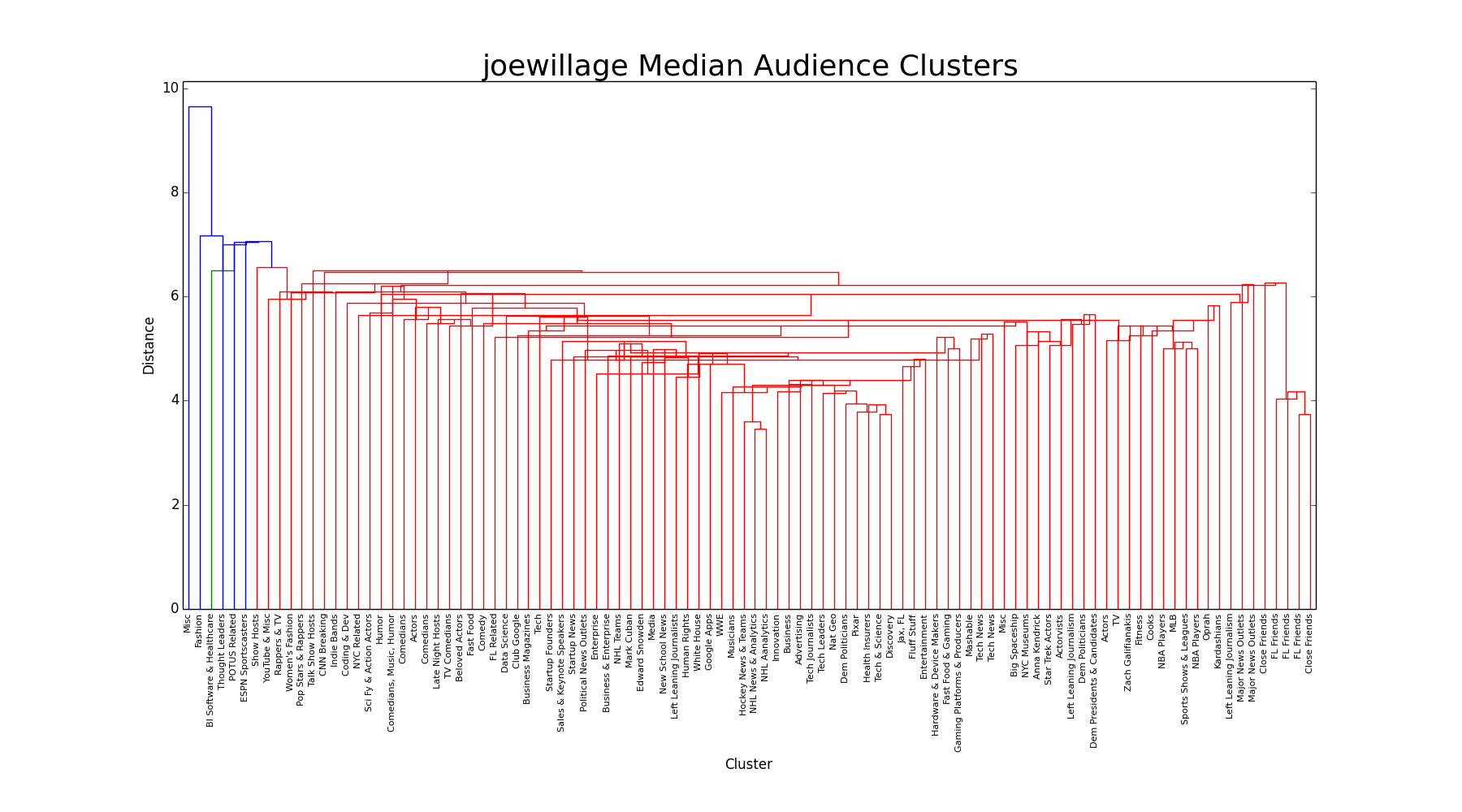
Similar to centroid, we see a lot of pre-clustered merges. Unlike k-median, which uses an observed point as the cluster center, the median linkage creates a cluster center in space, like centroid. The difference here is that median uses the average of the two centroids to create the new centroid, whereas the centroid linkage creates an entirely new centroid based on the original points in the two clusters. Like centroid, we notice a lot of singleton and small-cluster merges, with no distinct groups.
Single-Link

Single-link merges based on the closest members within each cluster. Perhaps this is too optimistic an approach in this situation. We see an extreme chaining effect picking up singletons and pairs of singletons.
Complete-Link
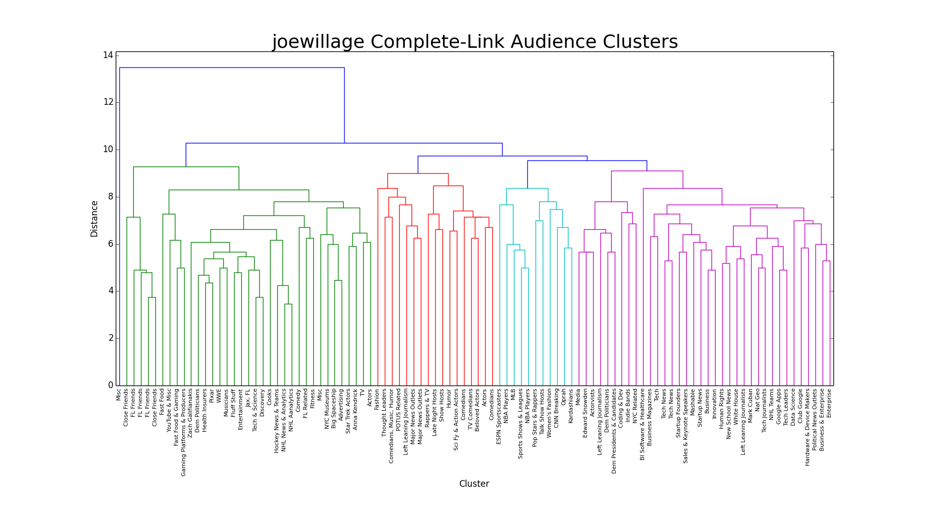
The complete-link dendrogram is the first linkage we see that actually looks like a good choice. There are four distinct groups, which seem to make sense as they merge (of course, 'making sense' isn't exactly what we're looking for. The clusters and correlations exist as they will. More often than not we'll observe clusters and merges that logically make sense, but there's no right or wrong here, because Twitter users that follow NBA players, for example, don't necessarily follow NBA teams). Instead of measuring the distance between the closest cluster members, as in single-link, complete-link measures the distance between the furthest members between clusters.
UPGMA
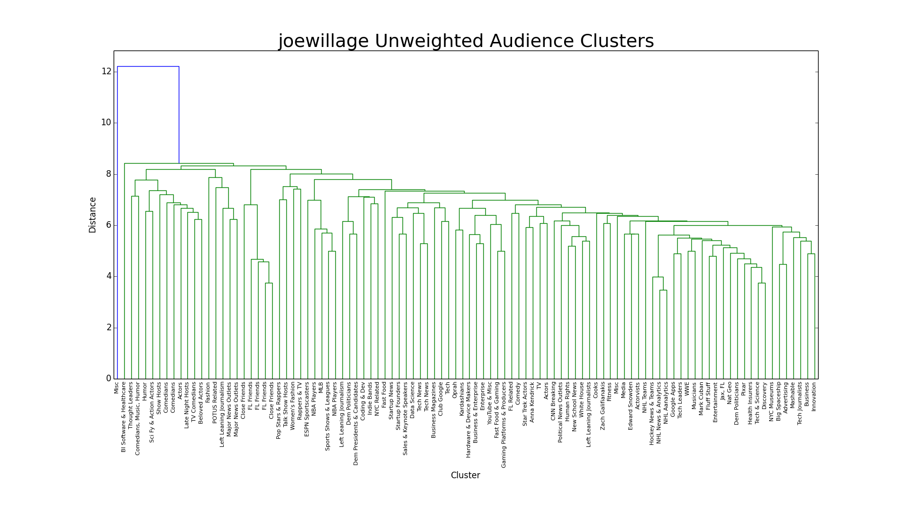
Referred to as 'average', this linkage compares the distance of the unweighted average distance between members of two clusters. It's a compromise between single and complete-link, and indeed that's what happens in the dendrogram. The groups aren't as distinct as complete-link, but the chaining isn't as extreme as single-linking.
WPGMA

This weighted version of UPGMA treats clusters of different sizes equally. So small clusters are weighted to act like large clusters. The weighting does a decent job, and we get a dendrogram that could pass as a feasible option. Compared to complete-link, however, the one large group in the middle is inferior. There's no cut-off point that would result in splitting up the large cluster without also creating many small clusters from the other groups.
Ward

The default linkage does in fact look like the best option. Ward's method works by minimizing the intra-cluster variance after clusters are merged. We end up with 5 distinct groups, with distances that lend themselves nicely to changing the cutoff point to create more granular groups, or larger groups. We'll stick with the current cutoff at 15, though.
As mentioned above, no metrics performed better than Euclidean for determining the distance, so we won't bother filling up the screen with dozens of graphs. But the Chebyshev distance was noteworthy. For each linkage, it produced a dendrogram that looked like this:

A Socialist uniformity, as you might expect from a metric named Chebyshev.
- https://dev.twitter.com/rest/reference/get/followers/ids ↩
- https://twitter.com/joewillage/status/804447346146746368 ↩
- https://docs.scipy.org/doc/scipy-0.18.1/reference/generated/scipy.cluster.hierarchy.linkage.html#scipy.cluster.hierarchy.linkage ↩
- "Best looking" is subjective, but in this application we're looking for a handful of distinct groups. There are other quantitative measurements of accuracy, such as the cophenetic correlation, which we looked at for each linkage/metric. ↩