
This is a first attempt at analyzing the NYC Street Tree Map data, specifically to find out which are the most tree-lined blocks.
library(ggmap)
library(knitr)
library(rjson)
library(dplyr)
Data is pulled from the NYC Street Tree Map site1. The call takes in diagonal points and creates an MBB using those points as the southwest and northeast corners. The coordinates below roughly describe a rectangle between the Manhattan bridge up to 8th and D. This is a reasonable area to start with while everything gets checked out and validated.
border.corner.sw.lat <- "40.71455760597046"
border.corner.sw.long <- "-73.99566650390625"
border.corner.ne.lat <- "40.723713744687295"
border.corner.ne.long <- "-73.97626876831055"

treemap.url <- paste("https://tree-map.nycgovparks.org/points",
              border.corner.sw.lat, border.corner.sw.long,
              border.corner.ne.lat, border.corner.ne.long,
              "undefined", "1", "2000", sep = "/")
raw <- fromJSON(file = treemap.url)
The json returned includes the latitude and longitude for each tree in the range, as well as the tree species, trunk diameter, and a few other data points. At this point the data is trimmed down from 1976 to a sample of 20 trees. These 20 will be used for validation.
samp <- raw$item[1:20]
samp[[1]]
## $id
## [1] 236951
##
## $lat
## [1] 40.72351
##
## $lng
## [1] -73.99377
##
## $species
## $species$id
## [1] 89
##
## $species$scientificName
## [1] "Acer campestre"
##
## $species$commonName
## [1] "Hedge Maple"
##
## $species$name
## [1] "Acer campestre - hedge maple"
##
## $species$code
## [1] "ACPL"
##
## $species$genusId
## [1] 31
##
## $species$imagePath
## NULL
##
## $species$libraryLink
## NULL
##
## $species$trees
## NULL
##
## $species$numberOfTrees
## NULL
##
## $species$color
## [1] "#76BF54"
##
## $species$description
## [1] "<p>Acer campestre, common name field maple, is a maple native to England and much of Europe, north to southern Scotland (where it is the only native maple), Denmark, Poland and Belarus, and also southwest Asia from Turkey to the Caucasus, and north Africa in the Atlas Mountains. In North America it is known as hedge maple and in Australia, it is sometimes called common maple.</p><p>It is a deciduous tree reaching 15-25 metres (49-82 ft) tall, with a trunk up to 1 metre (3 ft 3 in) in diameter, with finely fissured, often somewhat corky bark. The shoots are brown, with dark brown winter buds. The leaves are in opposite pairs, 5-16 centimetres (2.0-6.3 in) long (including the 3-9 centimetres (1.2-3.5 in) petiole) and 5-10 centimetres (2.0-3.9 in) broad, with five blunt, rounded lobes with a smooth margin. Usually monoecious, the flowers are produced in spring at the same time as the leaves open, yellow-green, in erect clusters 4-6 centimetres (1.6-2.4 in) across, and are insect-pollinated. The fruit is a samara with two winged achenes aligned at 180چ, each achene is 8-10 millimetres (0.31-0.39 in) wide, flat, with a 2 centimetres (0.79 in) wing.</p>\r"
##
##
## $stumpdiameter
## [1] 5The ArcGIS API2 is used to reverse geocode each data point. It returns the closest address to each tree.
gis.url <- paste0("http://geocode.arcgis.com/arcgis/rest/services/World/GeocodeServer/",
                 "reverseGeocode?f=json&location=")
treeMap <- lapply(samp, function(i) {
  address <- fromJSON(file = paste0(gis.url, i$lng, ",", i$lat))
  c(i$id, i$lat, i$lng, i$stumpdiameter, address$address$Match_addr)
  })

treeMap <- data.frame(matrix(unlist(treeMap), ncol = 5, byrow = TRUE), stringsAsFactors = FALSE)
treeMap$X5 <- gsub(", (New York|Knickerbocker), New York", "", treeMap$X5)
treeMap <- treeMap %>% separate(col = X5, into = c("address", "zip"), sep = ", ") %>%
                    separate(col = address, into = c("number", "street"), extra = "merge")
names(treeMap)[1:4] <- c("id", "lat", "lon", "stumpDiam")
treeMap$stumpDiam <- as.numeric(treeMap$stumpDiam)
treeMap$number <- as.numeric(treeMap$number)
treeMap$lat <- as.numeric(treeMap$lat)
treeMap$lon <- as.numeric(treeMap$lon)head(treeMap)## id lat lon stumpDiam number street zip
## 1 236951 40.72351 -73.99377 5 248 Elizabeth St 10012
## 2 248206 40.71810 -73.97664 8 140 Baruch Pl 10002
## 3 241049 40.71762 -73.99189 6 294 Grand St 10002
## 4 231671 40.72059 -73.98520 7 154 Stanton St 10002
## 5 238786 40.71582 -73.98400 10 10 Pitt St 10002
## 6 242345 40.72328 -73.97685 11 279 E 7th St 10009The next thing to do is build a reference table consisting of all the blocks, which are defined as street segments between two adjacent intersecting streets. The Census geocoding service3 provides start and end addresses for a block. Each tree has it's address looked up in the block table. If there is no row whose address range includes the tree, a new block will be added via the addBlock function.
census.url <- "http://geocoding.geo.census.gov/geocoder/locations/address?"
# seed block table with correct data types
blocks <- data.frame(id = 1, start = 222, end = 276, street = "Elizabeth St",
                     cross1 = "Prince St", cross1.lat = 40.722725, cross1.lon = -73.994156,
                     cross2 = "E Houston St", cross2.lat = 40.724434, cross2.lon = -73.99346,
                     zip = "10012", count = 0, stringsAsFactors = FALSE)
treeMap$blockId <- NULL
addBlockErr <- NULL
for (i in 1 : nrow(treeMap)) {
  x <- inner_join(treeMap[i, ], blocks, by = c("street" = "street", "zip" = "zip"))
  if (nrow(x) > 0) {
    y <- x$start <= unique(x$number) & x$end >= unique(x$number)
    if (sum(y)) {
      # Taking only first match, not differentiating between sides of street
      blocks[x[which(y)[1], "id.y"], "count"] <- blocks[x[which(y)[1], "id.y"], "count"] + 1
      treeMap[i, "blockId"] <-  x[which(y)[1], "id.y"]
    } else {
      blocks <- rbind(blocks,  addBlock(treeMap[i, ]))
      treeMap[i, "blockId"] <- max(blocks$id)
    }
  }
  else{
    blocks <- rbind(blocks,  addBlock(treeMap[i, ]))
    treeMap[i, "blockId"] <- max(blocks$id)
  }
}
addBlock <- function(tree) {
tryCatch({
census.parms <- paste0("street=", tree$number, "+",
gsub(" ", "+", tree$street), "&zip=", tree$zip,
"&city=new+york&state=NY&benchmark=9&format=json")
result <- fromJSON(file = paste0(census.url, census.parms))
from <- as.numeric(result$result$addressMatches[[1]]$addressComponents$fromAddress)
to <- as.numeric(result$result$addressMatches[[1]]$addressComponents$toAddress)
# geocode addresses at each side of block
from.parms <- paste0("street=", from, "+",
gsub(" ", "+", tree$street), "&zip=", tree$zip,
"&city=new+york&state=NY&benchmark=9&format=json")
to.parms <- paste0("street=", to, "+",
gsub(" ", "+", tree$street), "&zip=", tree$zip,
"&city=new+york&state=NY&benchmark=9&format=json")
fromCoord <- fromJSON(file = paste0(census.url, from.parms))
toCoord <- fromJSON(file = paste0(census.url, to.parms))
# lookup cross street
fromInt <- fromJSON(file = paste0(gis.url, fromCoord$result$addressMatches[[1]]$coordinates$x,
",", fromCoord$result$addressMatches[[1]]$coordinates$y,
"&returnIntersection=true"))
toInt <- fromJSON(file = paste0(gis.url, toCoord$result$addressMatches[[1]]$coordinates$x,
",", toCoord$result$addressMatches[[1]]$coordinates$y,
"&returnIntersection=true"))
if (grepl(tree$street, fromInt$address$Address)) {
cross1 <- gsub(tree$street, "", fromInt$address$Address)
cross1 <- gsub(" & ", "", cross1)
} else{
warning("Intersection does not include original street")
}
if (grepl(tree$street, toInt$address$Address)) {
cross2 <- gsub(tree$street, "", toInt$address$Address)
cross2 <- gsub(" & ", "", cross2)
} else{
warning("Intersection does not include original street")
}
# order so multiple segment entries will match
fromCross <- min(cross1, cross2)
toCross <- max(cross1, cross2)
# geocode intersection by names. More accurate point than start/end address
gis.url.parms1 <- URLencode(paste0(tree$street, " and ", fromCross, ", nyc"))
coords.cross1 <- paste0(gis.url.find, "&text=", gis.url.parms1)
gis.url.parms2 <- URLencode(paste0(tree$street, " and ", toCross, ", nyc"))
coords.cross2 <- paste0(gis.url.find, "&text=", gis.url.parms2)
coords.cross1 <- fromJSON(file = coords.cross1)
coords.cross2 <- fromJSON(file = coords.cross2)
tmp <- data.frame(id = nrow(blocks) + 1, start = min(from, to), end = max(from, to),
street = tree$street, cross1 = fromCross,
cross1.lat = coords.cross1$locations[[1]]$feature$geometry$y,
cross1.lon = coords.cross1$locations[[1]]$feature$geometry$x,
cross2 = toCross,
cross2.lat = coords.cross2$locations[[1]]$feature$geometry$y,
cross2.lon = coords.cross2$locations[[1]]$feature$geometry$x,
zip = tree$zip, count = 1, stringsAsFactors = FALSE)
tmp},
error = function(err) {
addBlockErr <<- c(addBlockErr, tree$id)
tmp <- data.frame(id = nrow(blocks) + 1, start = min(from, to), end = max(from, to),
street = tree$street,
cross1 = NA, cross1.lat = NA,cross1.lon = NA,
cross2 = NA, cross2.lat = NA,cross2.lon = NA,
zip = tree$zip, count = 1, stringsAsFactors = FALSE)
tmp
}
)
}This is a good point to check the validity of all the calls.
mymap <- get_map(location = "40.72017399459069,-73.98639034958494", zoom = 15,
                 maptype = "toner-lines")
blocks$int1 = paste(blocks$street, "&", blocks$cross1)
blocks2 <- data.frame(int2 = paste(blocks$street, "&", blocks$cross2),
                      cross2.lat = blocks$cross2.lat,
                      cross2.lon = blocks$cross2.lon)
g <-  ggmap(mymap) +
      theme_nothing() +
      geom_point(aes(x = cross1.lon, y = cross1.lat), data = blocks, color = "red", size = 5) +
      geom_text(aes(label = int1, x = cross1.lon, y = cross1.lat), data = blocks, color = "blue",
                check_overlap  = TRUE) +
      geom_point(aes(x = cross2.lon, y = cross2.lat), data = blocks2, color = "red",   size = 5) +
      geom_text(aes(label = int2, x = cross2.lon, y = cross2.lat), data = blocks2, color = "blue",
                 check_overlap  = TRUE)
g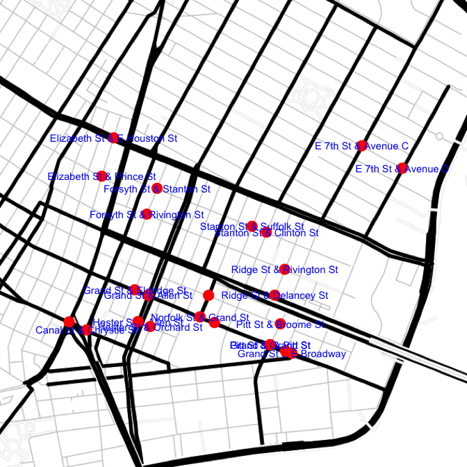
Everything is lining up correctly wrt intersections. A closer point-to-point inspection reveals minute discrepancies. For instance tree 216757 is reverse geocoded as being next to 464 Grand, but in reality is closer to 293 E Broadway, across the street. The tree will plot correctly on the map, but it won't fall into the correct bucket when aggregating trees by block. This is an acceptable margin of error at this point, but in the future, there are other options to explore reverse geocoding.
The same process is performed on the original data set of 1976 trees.
summary(blocks.les)## id start end street
## Min. : 1.00 Min. : -1.0 Min. : 7.00 Length:248
## 1st Qu.: 62.75 1st Qu.: 54.0 1st Qu.: 73.75 Class :character
## Median :124.50 Median :123.5 Median :147.00 Mode :character
## Mean :124.50 Mean :146.8 Mean :178.78
## 3rd Qu.:186.25 3rd Qu.:210.0 3rd Qu.:258.00
## Max. :248.00 Max. :900.0 Max. :934.00
##
## cross1 cross1.lat cross1.lon cross2
## Length:248 Min. :40.71 Min. :-74.00 Length:248
## Class :character 1st Qu.:40.72 1st Qu.:-73.99 Class :character
## Mode :character Median :40.72 Median :-73.99 Mode :character
## Mean :40.72 Mean :-73.99
## 3rd Qu.:40.72 3rd Qu.:-73.98
## Max. :40.72 Max. :-73.98
## NA's :23 NA's :23
## cross2.lat cross2.lon zip count
## Min. :40.71 Min. :-74.01 Length:248 Min. : 0.000
## 1st Qu.:40.72 1st Qu.:-73.99 Class :character 1st Qu.: 2.000
## Median :40.72 Median :-73.99 Mode :character Median : 5.000
## Mean :40.72 Mean :-73.99 Mean : 7.968
## 3rd Qu.:40.72 3rd Qu.:-73.98 3rd Qu.:11.000
## Max. :40.72 Max. :-73.97 Max. :36.000
## NA's :23 NA's :23incomplete <- blocks.les[!complete.cases(blocks.les),]
sum(incomplete$count)## [1] 186The resulting blocks table has 248 entries, with 23 NA's. Examining one of the NA's, 1 - 99 Willett St (id == 179), the first intersection returns correctly at Willett and Delancey. However, the other end of the block, 99 Willett, is incorrectly reverse geocoded up at Stanton St. Those incomplete blocks account for 186 trees, so it will be important to fill them in. To make the manual process easier, a subset of the addBlock function is broken out into the geocodeBlockEnds function.
gis.url.find <- "http://geocode.arcgis.com/arcgis/rest/services/World/GeocodeServer/find?f=json"
geocodeBlockEnds <- function(street, cross1, cross2){
  # given cross streets, add x and y coords

  # order so multiple segment entries will match
  fromCross <- min(cross1, cross2)
  toCross <- max(cross1, cross2)
  gis.url.parms1 <- URLencode(paste0(street, " and ", fromCross, ", nyc"))
  coords.cross1 <- paste0(gis.url.find, "&text=", gis.url.parms1)
  gis.url.parms2 <- URLencode(paste0(street, " and ", toCross, ", nyc"))
  coords.cross2 <- paste0(gis.url.find, "&text=", gis.url.parms2)
  coords.cross1 <- fromJSON(file = coords.cross1)
  coords.cross2 <- fromJSON(file = coords.cross2)
  l <- list(street = street,
            cross1 = list(
              street = cross1,
              y = as.numeric(coords.cross1$locations[[1]]$feature$geometry$y),
              x = as.numeric(coords.cross1$locations[[1]]$feature$geometry$x)
            ),
            cross2 = list(
              street = cross2,
              y = as.numeric(coords.cross2$locations[[1]]$feature$geometry$y),
              x = as.numeric(coords.cross2$locations[[1]]$feature$geometry$x)
            )
  )
  l
}

head(incomplete)
## id start end street cross1 cross1.lat cross1.lon cross2 cross2.lat
## 2 2 2 148 Baruch Pl <NA> NA NA <NA> NA
## 6 6 231 299 E 7th St <NA> NA NA <NA> NA
## 14 14 123 151 Canal St <NA> NA NA <NA> NA
## 25 25 700 798 E 5th St <NA> NA NA <NA> NA
## 29 29 260 398 E 3rd St <NA> NA NA <NA> NA
## 34 34 37 53 Avenue B <NA> NA NA <NA> NA
## cross2.lon zip count
## 2 NA 10002 14
## 6 NA 10009 25
## 14 NA 10002 2
## 25 NA 10009 31
## 29 NA 10009 36
## 34 NA 10009 4g <- geocodeBlockEnds("Baruch Pl", "Stanton St", "E Houston St")
blocks.les[blocks.les$id == 2, c(5:10)] <- c(g$cross1$street, g$cross1$y, g$cross2$x,
g$cross2$street, g$cross2$y, g$cross2$x)
blocks.les[blocks.les$id == 2, ]## id start end street cross1 cross1.lat cross1.lon
## 2 2 2 148 Baruch Pl Stanton St 40.7190615108811 -73.9768161138717
## cross2 cross2.lat cross2.lon zip count
## 2 E Houston St 40.7181138295907 -73.9768161138717 10002 14That assignment has to be repeated for each of the other 22 NAs, manually entering the correct cross streets. See corrections file for the full list of corrected segments. And some further error checking for bad segments...
same <- blocks.les[blocks.les$cross1 == blocks.les$cross2, ]
nrow(same)
## [1] 38After correcting these manually (see corrections file), the previously bad intersections look as follows
blocks.les$cross1.lat <- as.numeric(blocks.les$cross1.lat)
blocks.les$cross1.lon <- as.numeric(blocks.les$cross1.lon)
blocks.les$cross2.lat <- as.numeric(blocks.les$cross2.lat)
blocks.les$cross2.lon <- as.numeric(blocks.les$cross2.lon)

oldSame <- blocks.les[blocks.les$id %in% same$id, ]
oldSame$int1 = paste(oldSame$street, "&", oldSame$cross1)
oldSame2 <- data.frame(int2 = paste(oldSame$street, "&", oldSame$cross2),
                      cross2.lat = oldSame$cross2.lat,
                      cross2.lon = oldSame$cross2.lon)
g <-  ggmap(mymap) +
      theme_nothing() +
      geom_point(aes(x = cross1.lon, y = cross1.lat), data = oldSame, color = "red", size = 5) +
      geom_text(aes(label = int1, x = cross1.lon, y = cross1.lat), data = oldSame, color = "blue",
                check_overlap  = TRUE) +
      geom_point(aes(x = cross2.lon, y = cross2.lat), data = oldSame2, color = "red",   size = 5) +
      geom_text(aes(label = int2, x = cross2.lon, y = cross2.lat), data = oldSame2, color = "blue",
                 check_overlap  = TRUE)
g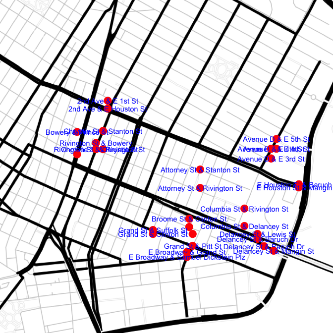
There's still some minute discrepancies, like the triangle of Grand/Clinton/E Broadway/Samuel Dickstein. But overall the new table is more accurate than the one with rows having the same cross street for both sides.
Blocks are collapsed so both sides of the street fall into a single block.
blocks.agg <- blocks.les %>% group_by(street, cross1, cross1.lat, cross1.lon, cross2,
                         cross2.lat, cross2.lon) %>%
  summarize(start = min(start), end = max(end), trees = sum(count)) %>%
  as.data.frame()
# Remove incomplete cases (which have a 0 count anyway)
blocks.agg <- blocks.agg[complete.cases(blocks.agg), ]
At this point it can be determined which blocks have the most trees.
head(blocks.agg[order(blocks.agg$trees, decreasing = TRUE), c(1, 2, 5, 10)], 10)## street cross1 cross2 trees
## 93 E 2nd St Avenue C E Houston St 36
## 96 E 3rd St Avenue C Avenue D 36
## 10 Allen St Rivington St Stanton St 34
## 105 E 6th St Avenue C Avenue D 33
## 99 E 4th St Avenue C Avenue D 32
## 9 Allen St Grand St Hester St 31
## 102 E 5th St Avenue B Avenue C 31
## 103 E 5th St Avenue C Avenue D 31
## 146 Forsyth St Rivington St Stanton St 30
## 91 E 2nd St Avenue A Avenue B 28Not surprisingly, the long blocks between avenues have the highest count of trees, all of which are in the East Village.
map.evill <- get_map(location = "40.7228765,-73.9805015", zoom = 17, maptype = "toner-lines")
blocks.agg$int1 <- paste(blocks.agg$street, "&", blocks.agg$cross1)

g <- ggmap(map.evill) +
  geom_point(data = treeMap, aes(x = lon, y = lat, size = stumpDiam, color = stumpDiam),
             alpha = 0.35) +
  scale_size(range = c(5, 7)) +
  theme_nothing() +
  scale_color_continuous(low = "chartreuse", high = "chartreuse4") +
  geom_text(aes(label = int1, x = cross1.lon, y = cross1.lat), data = blocks.agg, color = "red",
                fontface = "bold", check_overlap  = TRUE)
blocks.agg$int1 <- NULL
g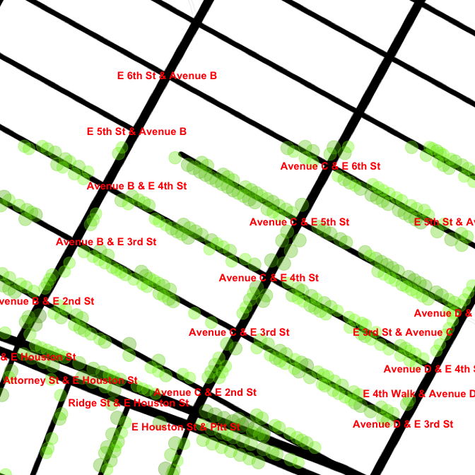
"Which block is the most tree-lined" can be answered now, but that answer is biased. Longer blocks have an advantage. A more accurate measure would be trees per meter (TPM). To determine the distance of a block, the Great-circle distance is used with the Haversine formula.
deg2rad <- function(deg) return(deg * pi / 180)

gcd <- function(long1, lat1, long2, lat2) {
  # Computes the great-circle distance between two points using the haversine formula
  #
  # Args:
  #   long1:  Longitude of first point in decimal degrees
  #   lat2:   Latitude of first point in decimal degrees
  #   long2:  Longitude of first point in decimal degrees
  #   lat2:   Latitude of second point in decimal degrees
  #
  # Returns:
  #   The distance in meters

  long1 <- deg2rad(long1)
  lat1 <- deg2rad(lat1)
  long2 <- deg2rad(long2)
  lat2 <- deg2rad(lat2)
  r <- 6371000
  long.delt <- (long2 - long1)
  lat.delt <- (lat2 - lat1)
  a <- sin(lat.delt / 2)^2 + cos(lat1) * cos(lat2) * sin(long.delt / 2)^2
  c <- 2 * atan2(sqrt(a), sqrt(1 - a))
  r * c
}
blocks.agg$distance <- NULL
for (i in 1:nrow(blocks.agg)) {
d <- gcd(blocks.agg[i, "cross1.lon"],
blocks.agg[i, "cross1.lat"],
blocks.agg[i, "cross2.lon"],
blocks.agg[i, "cross2.lat"])
blocks.agg[i, "distance"] <- d
}
blocks.agg$tpm <- blocks.agg$trees / blocks.agg$distance
head(blocks.agg[order(blocks.agg$tpm, decreasing = TRUE), c(1, 2, 5, 10:12)], 10)## street cross1 cross2 trees distance tpm
## 150 Grand St Clinton St Suffolk St 23 27.57541 0.8340763
## 96 E 3rd St Avenue C Avenue D 36 112.27125 0.3206520
## 105 E 6th St Avenue C Avenue D 33 111.28635 0.2965323
## 52 Broome St Pitt St Ridge St 23 79.22609 0.2903084
## 103 E 5th St Avenue C Avenue D 31 111.28635 0.2785607
## 93 E 2nd St Avenue C E Houston St 36 132.35417 0.2719975
## 120 E Houston St Norfolk St Suffolk St 20 77.31952 0.2586669
## 10 Allen St Rivington St Stanton St 34 136.65020 0.2488105
## 159 Grand St Pitt St Willett St 19 82.56288 0.2301276
## 106 E 7th St Avenue C Avenue D 25 111.28635 0.2246457This gives an answer, but how valid is it? The preliminary checks above looked reasonably good, but can the block of Grand between Clinton and Suffolk really have so many more trees per meter than any other block? A closer inspection can isolate the trees mapped to just that block.
blocks.les[blocks.les$street == "Grand St" & blocks.les$cross1 == "Clinton St",]## id start end street cross1 cross1.lat cross1.lon cross2
## 35 35 393 411 Grand St Clinton St 40.71595 -73.98753 Suffolk St
## 204 204 430 440 Grand St Clinton St 40.71595 -73.98426 Pitt St
## 209 209 426 428 Grand St Clinton St 40.71595 -73.98670 Ridge St
## cross2.lat cross2.lon zip count
## 35 40.71620 -73.98753 10002 23
## 204 40.71521 -73.98426 10002 4
## 209 40.71543 -73.98500 10002 4treeMap[treeMap$blockId == 35, ]## lat lon stumpDiam number street zip id blockId
## 62 40.71597 -73.98678 3 410 Grand St 10002 159576 35
## 747 40.71578 -73.98653 26 410 Grand St 10002 202497 35
## 937 40.71542 -73.98712 8 410 Grand St 10002 135487 35
## 945 40.71554 -73.98707 14 410 Grand St 10002 187690 35
## 959 40.71533 -73.98694 7 410 Grand St 10002 218980 35
## 1081 40.71544 -73.98689 5 410 Grand St 10002 270636 35
## 1147 40.71590 -73.98623 3 410 Grand St 10002 230817 35
## 1149 40.71553 -73.98569 3 409 Grand St 10002 233518 35
## 1152 40.71566 -73.98613 3 410 Grand St 10002 235203 35
## 1154 40.71596 -73.98642 3 410 Grand St 10002 239903 35
## 1156 40.71623 -73.98649 4 410 Grand St 10002 240885 35
## 1159 40.71593 -73.98632 3 410 Grand St 10002 245908 35
## 1176 40.71618 -73.98651 4 410 Grand St 10002 280045 35
## 1195 40.71573 -73.98697 4 410 Grand St 10002 141254 35
## 1197 40.71564 -73.98702 5 410 Grand St 10002 157304 35
## 1200 40.71580 -73.98693 4 410 Grand St 10002 188910 35
## 1294 40.71611 -73.98655 3 410 Grand St 10002 286539 35
## 1593 40.71577 -73.98649 28 410 Grand St 10002 154294 35
## 1596 40.71574 -73.98675 28 410 Grand St 10002 156627 35
## 1690 40.71530 -73.98717 12 410 Grand St 10002 165907 35
## 1695 40.71565 -73.98679 27 410 Grand St 10002 247302 35
## 1696 40.71554 -73.98684 27 410 Grand St 10002 265252 35
## 1755 40.71549 -73.98557 6 409 Grand St 10002 260669 35map.sewardPark <- get_map(location = "40.71597,-73.9889687", zoom = 17, maptype = "toner-lines")
ggmap(map.sewardPark) +
geom_point(data = treeMap[treeMap$blockId == 35,],
aes(x = lon, y = lat, size = stumpDiam), alpha = 0.35, color = "chartreuse") +
scale_size(range = c(5, 7)) +
theme_nothing()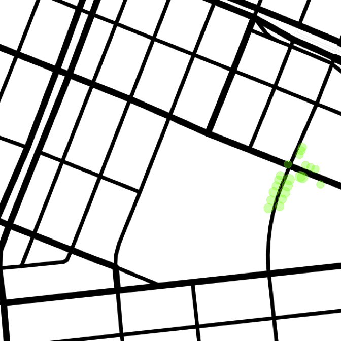
The majority of the trees actually lie along Clinton, although they were coded at 410 Grand. This highlights the roughness of geocoding coordinates to addresses, and the limitations of the tools available. The manual work using the above procedures make it unfeasible to report over the entire city, which includes more than 300,000 trees. At this point, there's enough certainty to say that the blocks from this sample data set with the most trees per meter (and trees in general) are between Avenues C and D. Here is the complete map of all the trees from the original request.
g <- ggmap(mymap) +
  geom_point(data = treeMap,
             aes(x = lon, y = lat, size = stumpDiam, color = stumpDiam),
             alpha = 0.35) +
  scale_size(range = c(5, 7)) +
  theme_nothing() +
  scale_color_continuous(low = "chartreuse", high = "chartreuse4")
g
New York City Street Tree Map Beta
Interactive map to view details from a city-wide to a single tree level. No official API
https://tree-map.nycgovparks.org/points/<SW lat>/<SW lng>/<NE lat>/<NE lng>/undefined/ <start tree>/<end tree>
View details of a specific tree, including closest address:
https://tree-map.nycgovparks.org/tree/full/<tree-id from points json>
Browser-based map:
https://tree-map.nycgovparks.org/ ↩ArcGIS REST API: World Geocoding Service
ReverseGeocode returns the closest address to a given lat/lng location
http://developers.arcgis.com/rest/geocode/api-reference/geocoding-reverse-geocode.htm
The Find operation geocodes input and can handle intersections
https://developers.arcgis.com/rest/geocode/api-reference/geocoding-find.htm ↩US Census Geocoding Services
Geocodes addresses and also returns the range of addresses on the block of input http://geocoding.geo.census.gov/geocoder/Geocoding_Services_API.html
Also available as browser-based app: http://geocoding.geo.census.gov/geocoder/locations/address ↩